FastMetrics, Part 3 - Maximizing Resolution

Background

Welcome to Part 3 of the Monitoring Fast Metric series! From a raw tiny server instance we built a scalable logging server, and then taught our client how to aggregate and send endless raw data for us. Job done, might as well deploy and jump straight to the analysis - with that much, you’d already be doing better than most of the sites and apps out there that either log way too much or miss out on the important fast moving information they need!

I think we can do better, though. Going back to the mind map, we’re still caring about data we aren’t interested in, and we might miss out on the rare things that seem to be pretty frequent:

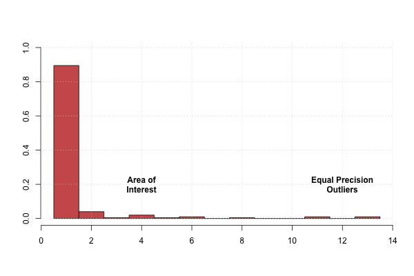
That’s actually already pretty awesome, and feel free to jump ahead to the analysis, or take a segue through mapping IPs to ASNs. FlatHistograms already do a reasonable job of aggregating data, but they give equal resolution to every bin that is being logged, which doesn’t exactly match our desires. In the case of latencies, for example, we’re paying as much attention to the area of interest as we are to the outliers:

What is to be done?

Today’s Agenda

When aggregating the data, there was no reason to assume that we needed to choose the bins to be equally spaced. To take a delay example in a web browser, I’m going to look at transactionTime that we captured last time, which measures how long it takes from a browser firing off a request to that data sitting on the device, ready for consumption. If we assume that our requests take between 0 (cache hits) to 2 seconds to complete, we’re less interested in exactly how long they take when they’re past 10 seconds - something went wrong with the CDN or the code, but we don’t need to know exactly how long those requests took when they’re that far out. We really only need to recognize how often they happened.

With the FlatHistogram implementation, to be able to see things over that range, we would need to set the range from 0 to something above 10 (say 20). If we wanted to count the delays in seconds, we’d need 20 bins to get enough resolution, but then we’re getting the same precision in the range from 10-20 as we are from 0-10, where we were less interested. If we want more resolution around the area of interest, say for values less than 5, we would still need to increase the number of bins everywhere to get the finer grain, or we’d need to go to quarter second intervals, where we would need 80 bins!

That leaves us with two options:

1. Bump up the number of bins and deal with increased amounts of data, or
2. Choose a different binning strategy.

As an additional caveat, I will avoid using any pre-arranged binning strategies since that complicates the implementations for the rest of that data’s life. In practice, with how fast things tend to change, I want to prefer more flexible self-describing solutions that can be applied over vastly differing scales quickly with very little maintenance overhead, which leaves only binning that can be calculated at runtime from a simple description, or the raw data itself.

There has, fortunately, been a lot of research on different binning strategies, and today I will show you one that is used by Chrome, Firefox, and Netflix, which incurs little to no additional CPU cost over the FlatHistogram strategy - the ExponentialHistogram.

For more CPU and memory, we can do even better with more complex techniques, but I saw implementation issues with the lowest end hardware I was supporting at Netflix, so we’ll leave that for another article, if there’s interest.

The Pieces

I. Calculating the exponentially spaced buckets Using the code from the previous article, we can get a FlatHistogram from 0 to 20 with a bucket for each number, with:

var hist = new FlatHistogram("transactionTime", 0, 200, 20);

which creates a structure that looks like this as JSON:

{
 "name":"transactionTime",
 "layout":"F/0/200/20",
 "data":{
  "10":0,"20":0,"30":0,"40":0,
  "50":0,"60":0,"70":0,"80":0,
  "90":0,"100":0,"110":0,"120":0,
  "130":0,"140":0,"150":0,"160":0,
  "170":0,"180":0,"190":0,"200":0
  }
}

Now what if we still kept 20 buckets, but wanted the numbers near the top to be much further apart than those towards the bottom? We can observe that we need coverage over the range from 0 to 200 (range of 200), but keep sliding the buckets further apart the closer we get to 200 by using increasing roots of the range. To do this, let’s swap out the initializeBucketRanges from FlatHistograms with some new math:

// Adapted from: chromium/src/base/metrics/histogram.cc
function initializeBucketRanges(minimum, maximum, bucket_count) {
    var ranges = [];
    var log_max = Math.log(maximum);
    var log_ratio;
    var log_next;
    var bucket_index = 1;
    var current = minimum;
    var buckets = [];

    // always add a zero bucket for negatives / errors
    buckets.push(0);
    if (current > 0) { buckets.push(current); }

    while (bucket_count > ++bucket_index) {
        var log_current = Math.log(current);
        // Calculate the count'th root of the range.
        log_ratio = (log_max - log_current) /
            (bucket_count - bucket_index);
        // See where the next bucket would start.
        log_next = log_current + log_ratio;
        var next = Math.round(Math.exp(log_next));
        if (next > current) { current = next; }
        else { ++current; }
        buckets.push(current);
    }

    return buckets;
}

then we just need to change the FlatHistogram names to ExponentialHistogram in the rest of the code, and change the layout to use the name “E” instead of “F”. You could also get fancy and just replace the initializeBucketRanges function on FlatHistogram's prototype and rename the class, but I’ll leave that to you for now.

II. Comparing the resolutions of interest What sort of histogram do we get when we use the same range and bucket counts?

var hist2 = new ExponentialHistogram("transactionTime", 0, 200, 20);

which creates a structure that looks like this in JSON:

{
 "name":"transactionTime",
 "layout":"E/0/200/20",
 "data":{
  "1":0,"2":0,"3":0,"4":0,
  "5":0,"7":0,"9":0,"12":0,
  "16":0,"21":0,"28":0,
  "37":0,"49":0,"65":0,"86":0,
  "114":0,"151":0,"200":0
 }
}

Close to 0, the buckets are very close together, while they spread out very far near 200. If we put them on the same scale:

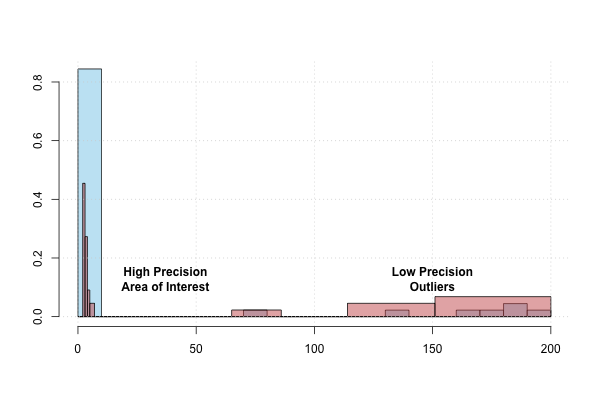
Success! In the case of network delays, such as we discussed before, now we have a lot more resolution towards the area of interest, and significantly less at the outliers. This matches our original intention, since the exact magnitude of an outlier is probably less interesting to us as opposed to just knowing that or how often it happened.

III. Filtering out There is one more useful optimization we can make to cut down on the amount of data that we’re logging. Over short time intervals, such as during a user’s session on a website, many of the buckets will not be filled with any counts at all. This leaves us with a lot of zeros in the data, such as in this example of transactionTime counts harvested from a far away website:

{
 "name":"transactionTime",
 "layout":"E/0/200/20",
 "data":{
  "1":0,"2":1,"3":0,"4":0,
  "5":0,"7":0,"9":1,"12":1,
  "16":0,"21":1,"28":3,
  "37":2,"49":3,"65":3,"86":7,
  "114":0,"151":2,"200":0
 }
}

If we include the layout in the payload (as we have been), then we can always reconstruct which bins were filtered out based on the original parameters, so there’s no need to log a whole bunch of bins with no counts in them. Let’s apply a simple filter to the log data to remove zero counts:

{
 "name":"transactionTime",
 "layout":"E/0/200/20",
 "data":{
  "2":1,"9":1,"12":1,"21":1,
  "28":3,"37":2,"49":3,"65":3,
  "86":7,"151":2
 }
}

So now the stringify function looks like this (leaving both options with the suppressZeros boolean trap):

    stringify: function stringify(suppressZeros) {
        var i, currentCount, totalNonzeroCounts = 0;
        var data = {};

        for (i = 1 ; i < this.buckets.length ; ++i) {
            currentCount = this.counts[i-1];
            if (suppressZeros === true) {
                if (currentCount > 0) {
                    totalNonzeroCounts += 1;
                    data[this.buckets[i]] = currentCount;
                }
            } else {
                data[this.buckets[i]] = currentCount;
            }
        }

        // TODO: filter out records with empty data
        return JSON.stringify({
                name: this.name,
                layout: this.layout,
                data: data
            });
    },

Additionally we can also drop any record that has no counts at all in the data field, assuming we aren’t interested in receiving heartbeats from clients. Cutting down on the amount of data being logged at the client will reduce how much filtering is needed up at the server.

Next Time

We have now improved our resolution in the areas of the data where we are most interested, and blown away the chaff from the rest of the data. In the next article, we will investigate mapping an IP address to an ASN, a useful dimension to roll up against when looking for common network experiences among users, a useful ingredient for our final analysis.